Using SMUP
You use the Smup class to produce smups (Stable Matchings Useless Pictures). A smup is built in two steps:
A compute phase generates the topology of the smup;
A display phase handles the actual drawing/saving.
The following is a minimal code to produce a smup.
[1]:
from smup import Smup
smup = Smup()
smup.compute()
smup.display()
Computational parameters
For computing, you can adjust:
the distance function used;
the size of the picture;
the number of sites.
Distance functions
Norms
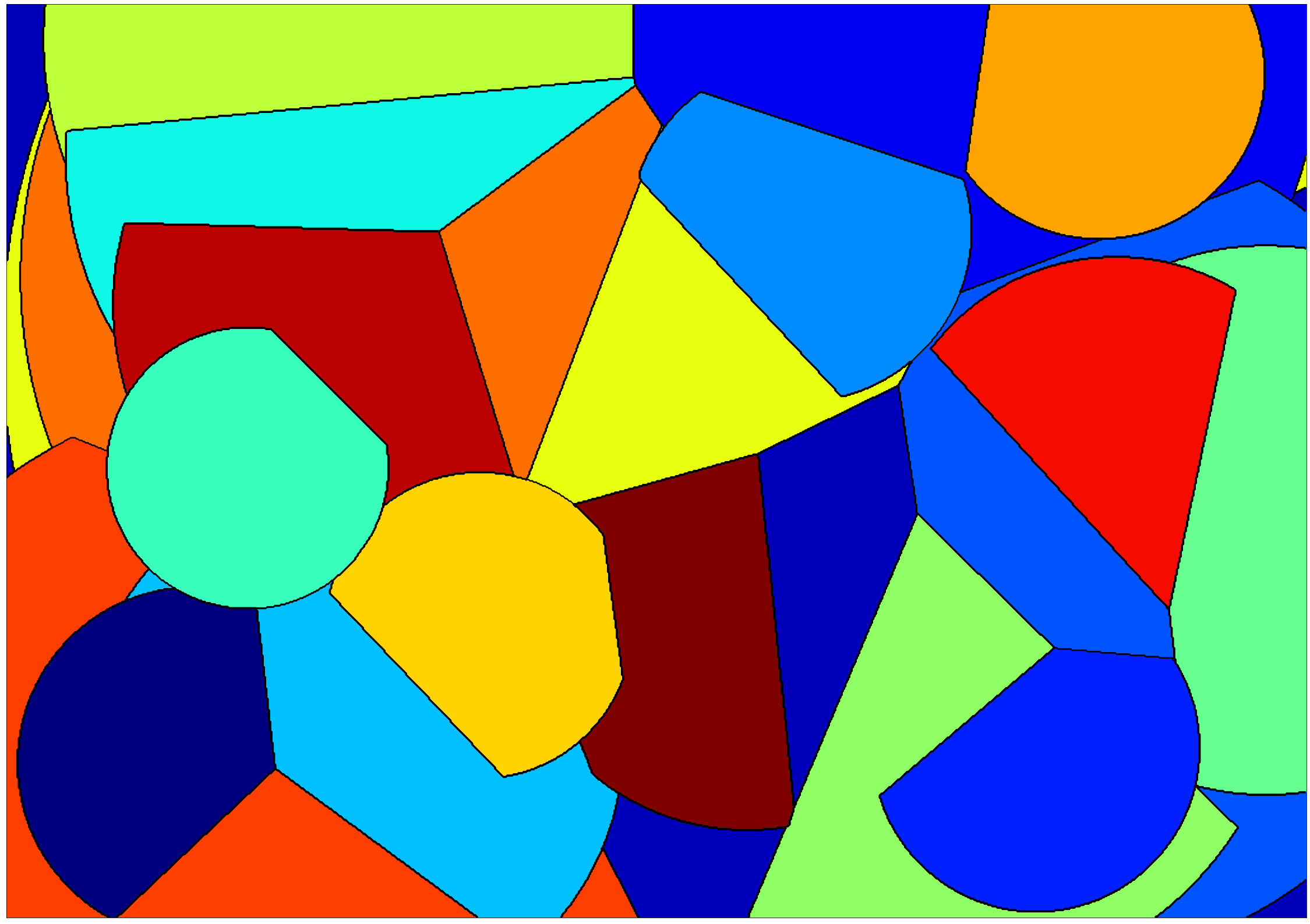
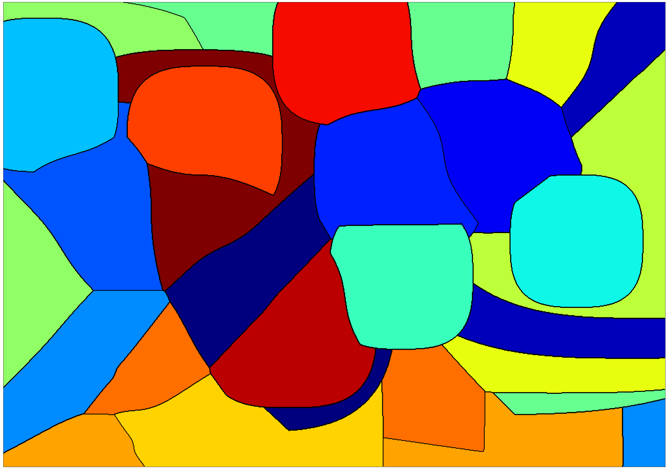
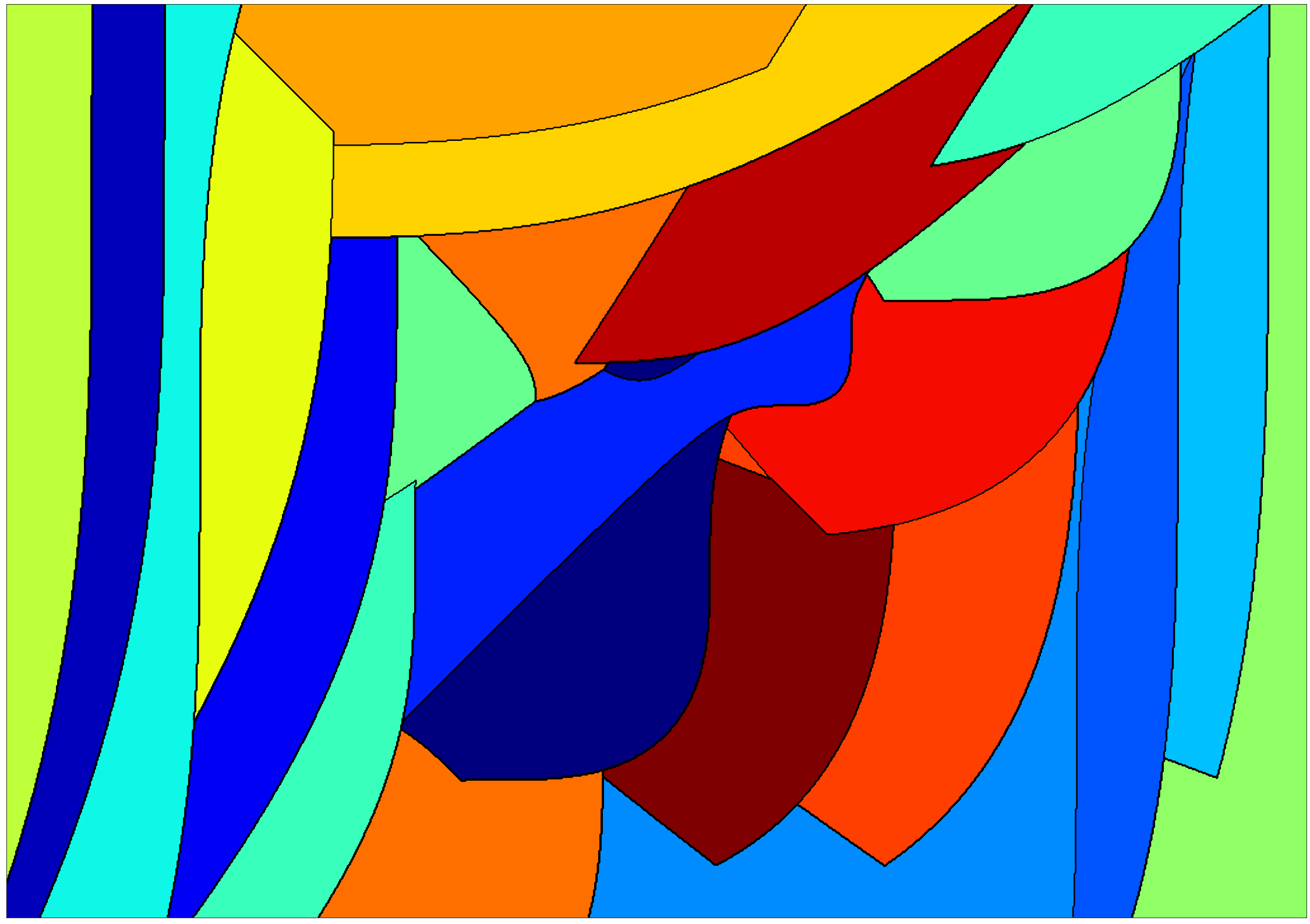
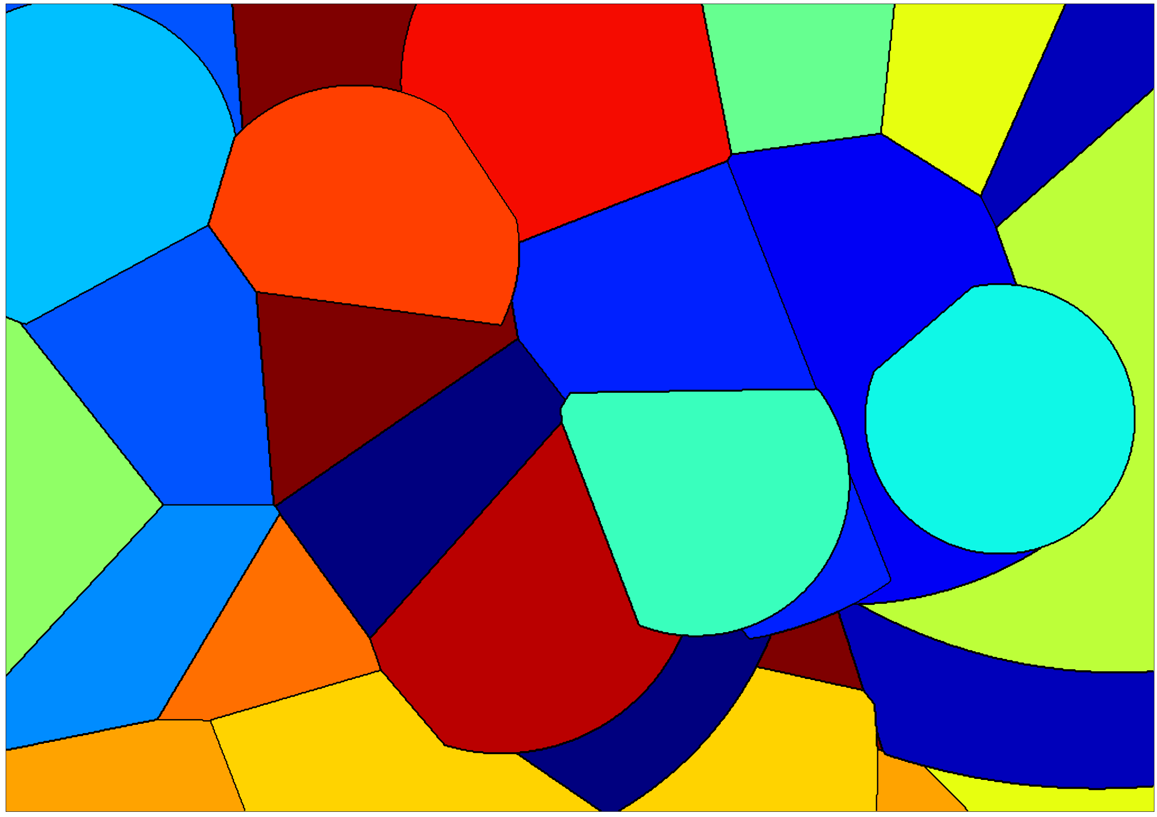
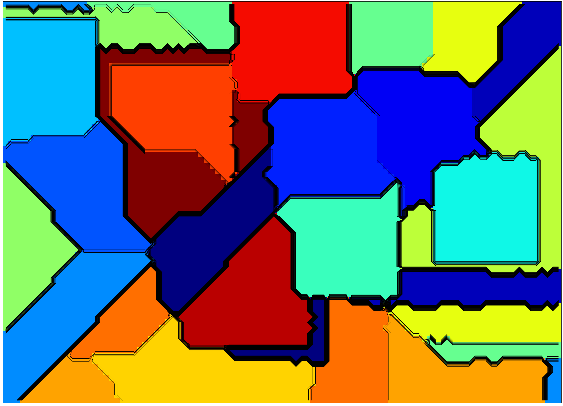
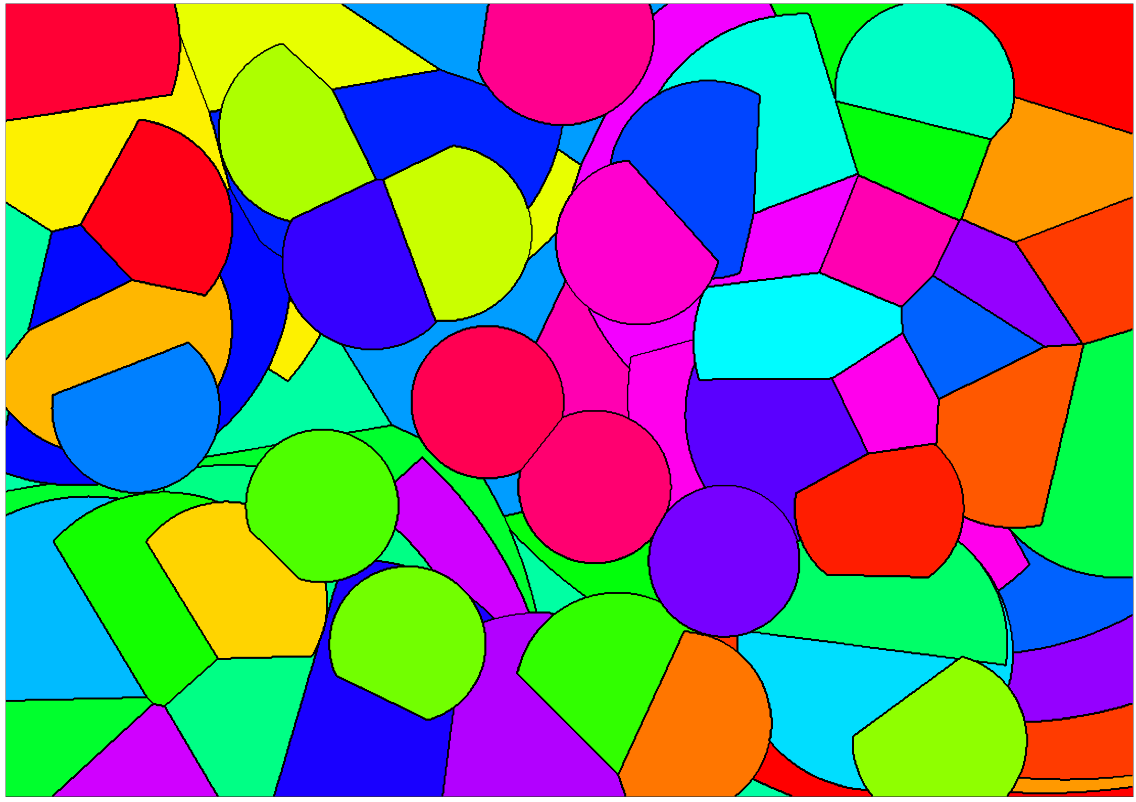
By default, the smup will use the Euclidian distance (norm 2), which will shape the sites as (partial) circles. Note the use of a random seed in the code below, which will allows to fix the location of the sites and see the effect of the norm.
[2]:
smup.compute(seed=42)
smup.display()
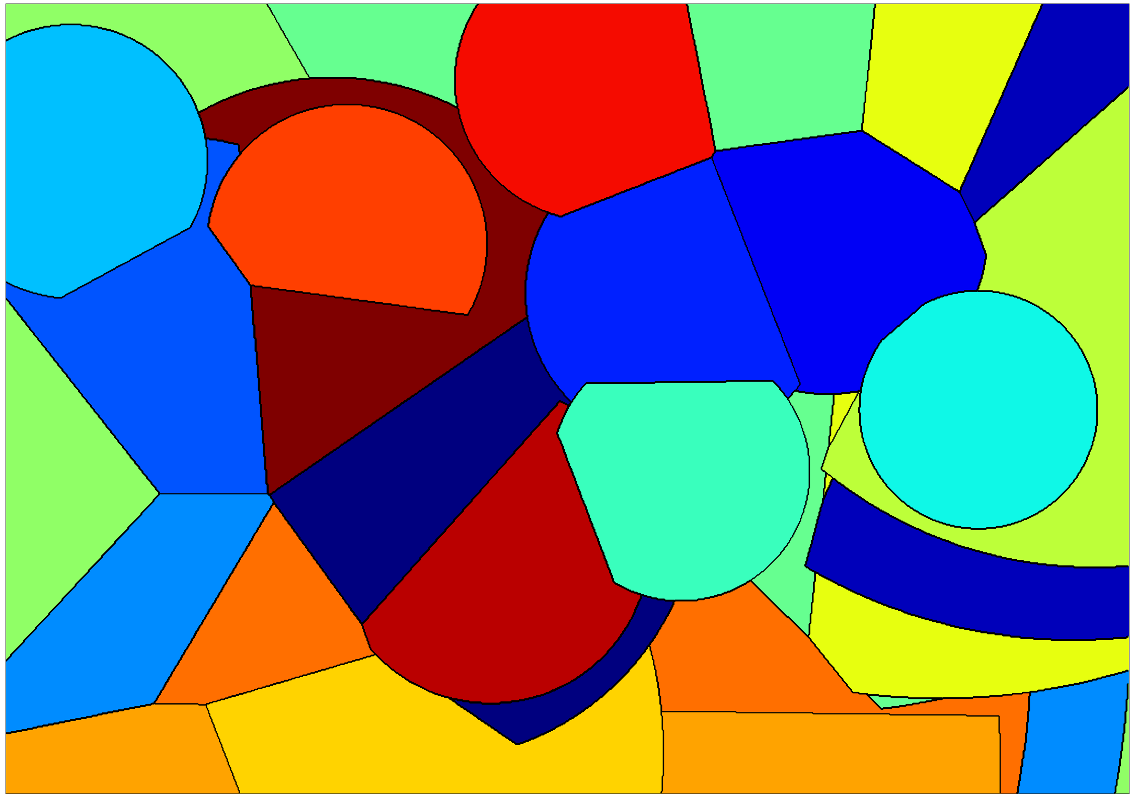
The Manhattan distance (norm 1) will shape the sites as (partial) diamonds. Note the use of a random seed in the code below, which will allows to fix the location of the sites and see the effect of the norm.
[3]:
smup.compute(norm=1, seed=42)
smup.display()
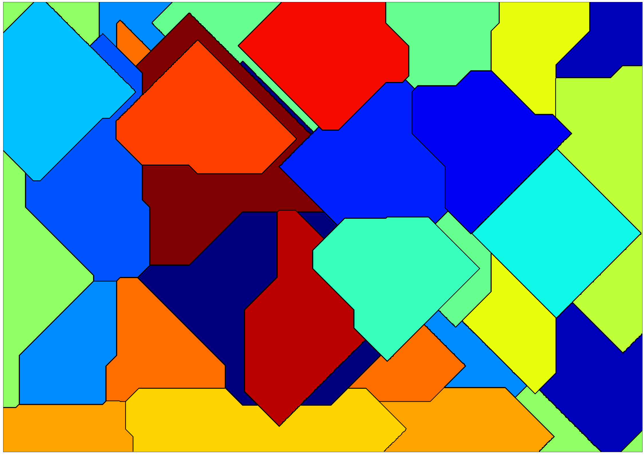
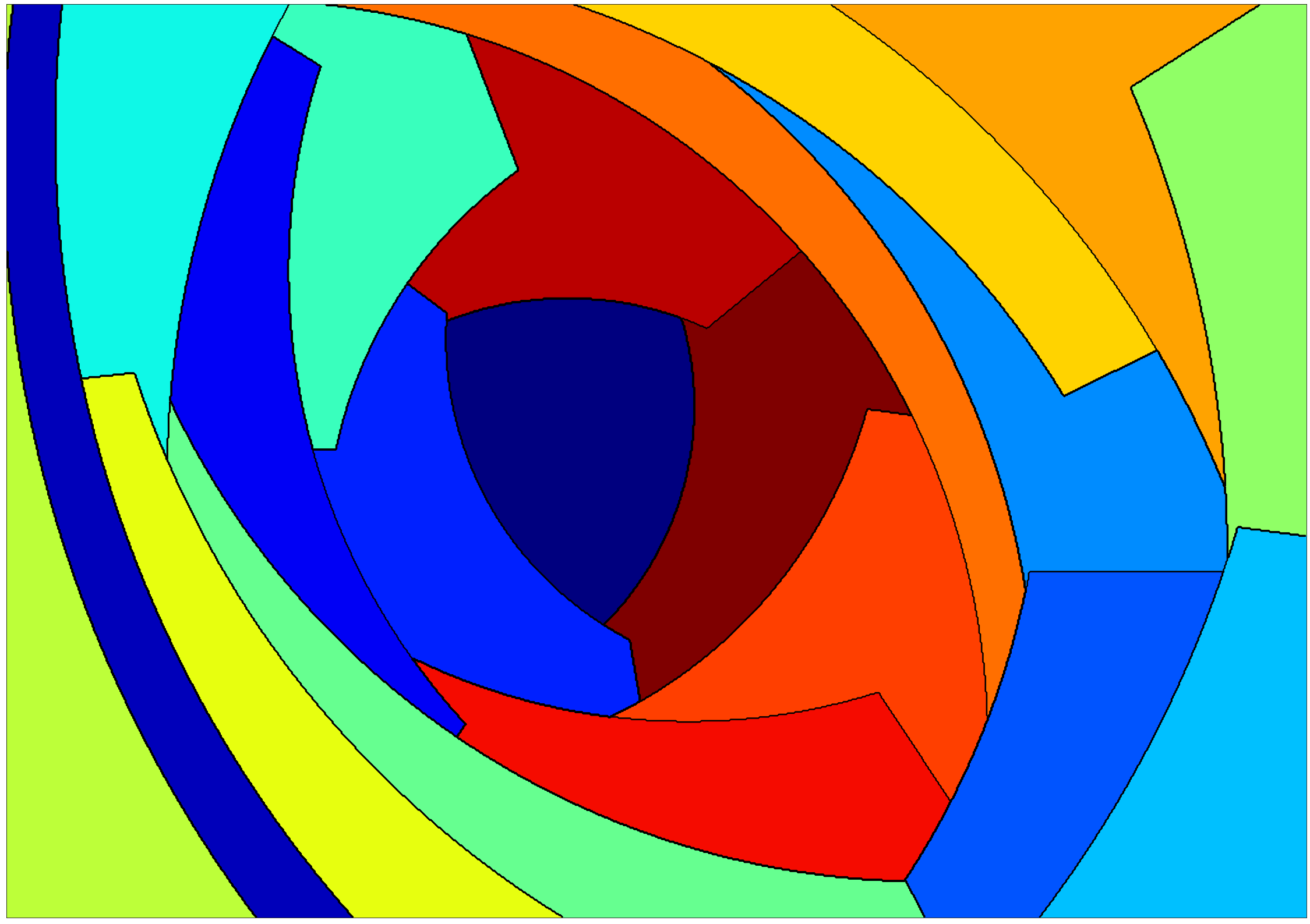
The infinite norm will shape the sites as (partial) squares. Note the use of a random seed in the code below, which will allows to fix the location of the sites and see the effect of the norm.
[4]:
smup.compute(norm="inf", seed=42)
smup.display()
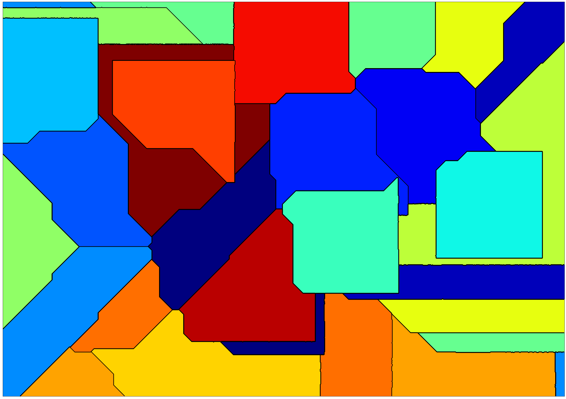
You can also an arbitrary float for the norm (corresponds to Hölder’s p-norm). 3-norm:
[5]:
smup.compute(norm=3, seed=42)
smup.display()
1.5 norm:
[6]:
smup.compute(norm=1.5, seed=42)
smup.display()
Arbitrary functions
If you use a value smaller than 1, the result do not correspond to an actual norm (no convexity) and the pictures are even more chaotic.
[7]:
smup.compute(norm=.5, seed=42)
smup.display()
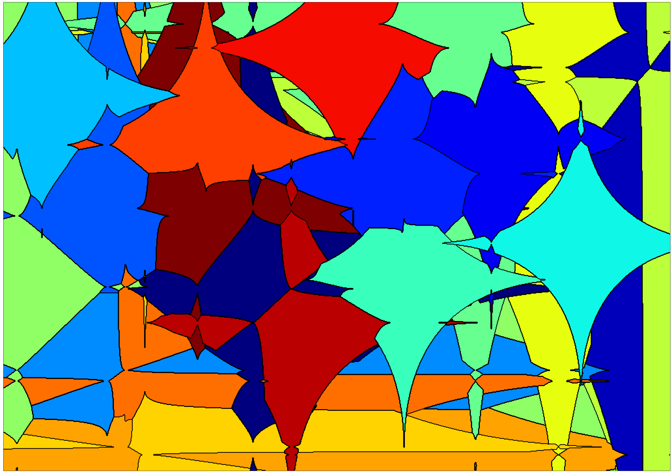
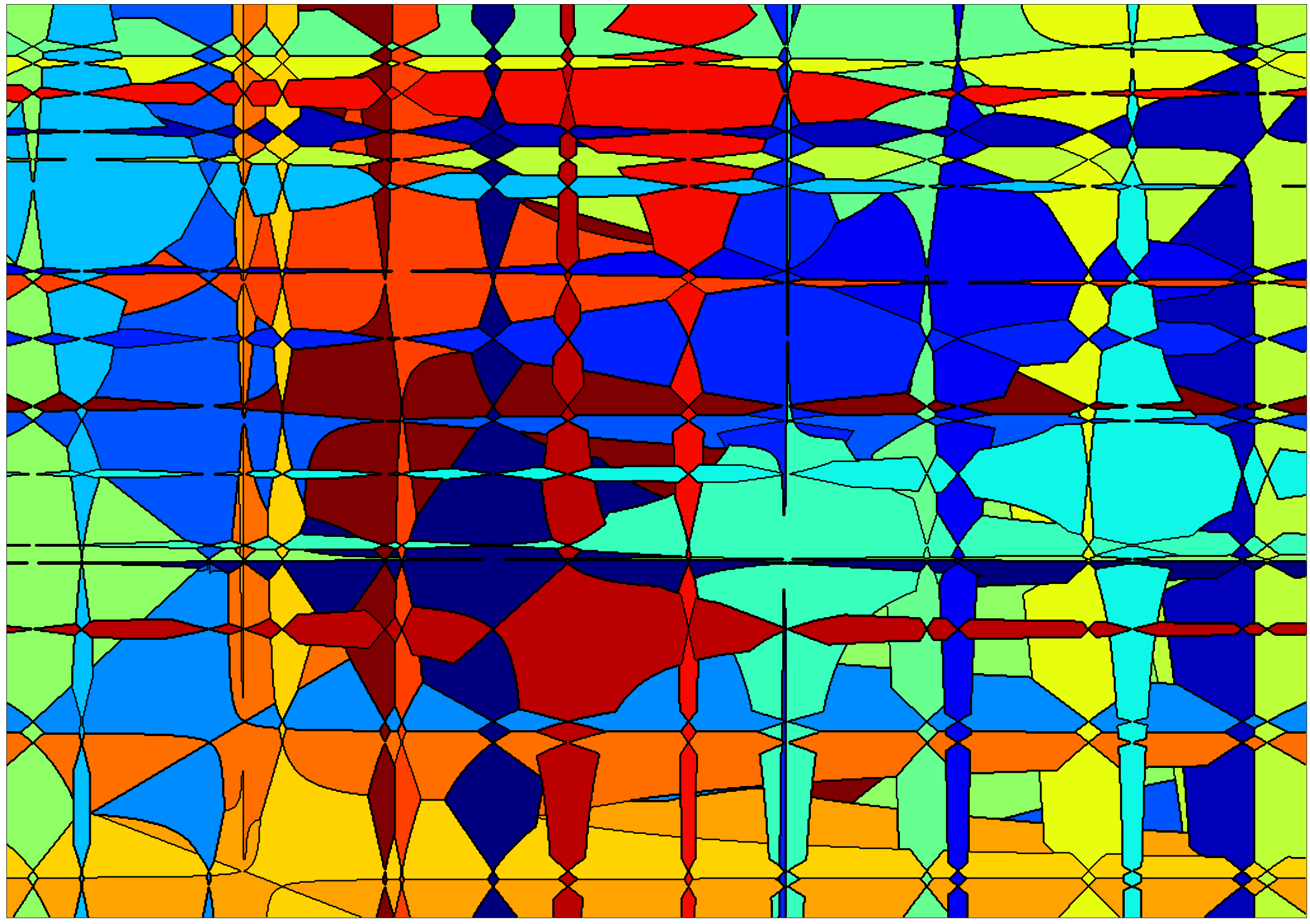
If you want to go further into that direction, you can input an arbitrary distance function, which may not be a distance at all! See the examples below:
[8]:
import numpy as np
def log_weight(center, points):
    return np.log(np.abs(points[0, :] - center[0])) + np.log(np.abs(points[1, :] - center[1]))

smup.compute(norm=log_weight, seed=42)
smup.display()
[9]:
def cubic(center, points):
    return (points[0, :] - center[0])**3 + (points[1, :] - center[1])**3

smup.compute(norm=cubic, seed=42)
smup.display()
[10]:
from smup.smup import dist_2

def repulsive(center, points):
    return -dist_2(center, points)

smup.compute(norm=repulsive, seed=42)
smup.display()
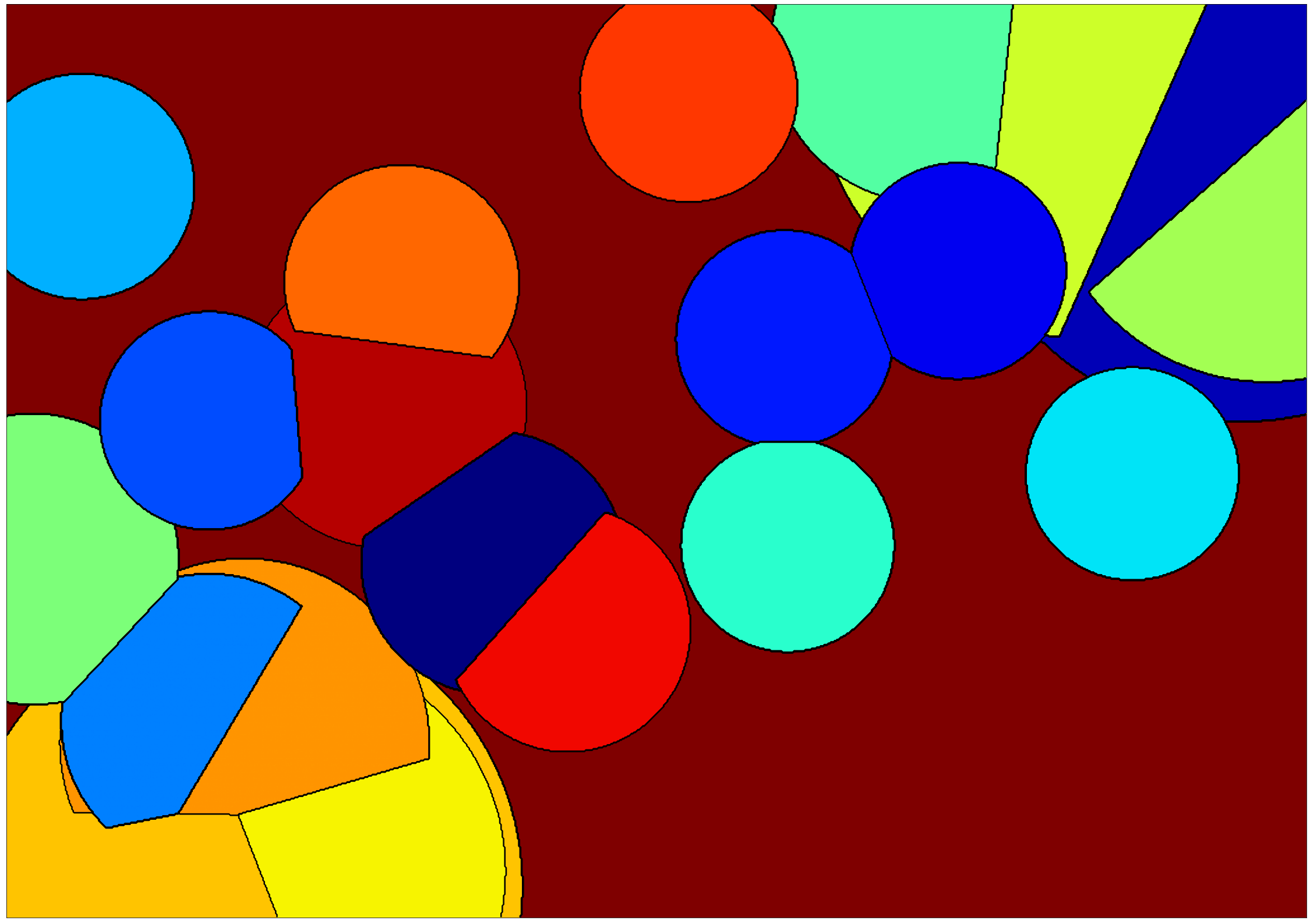
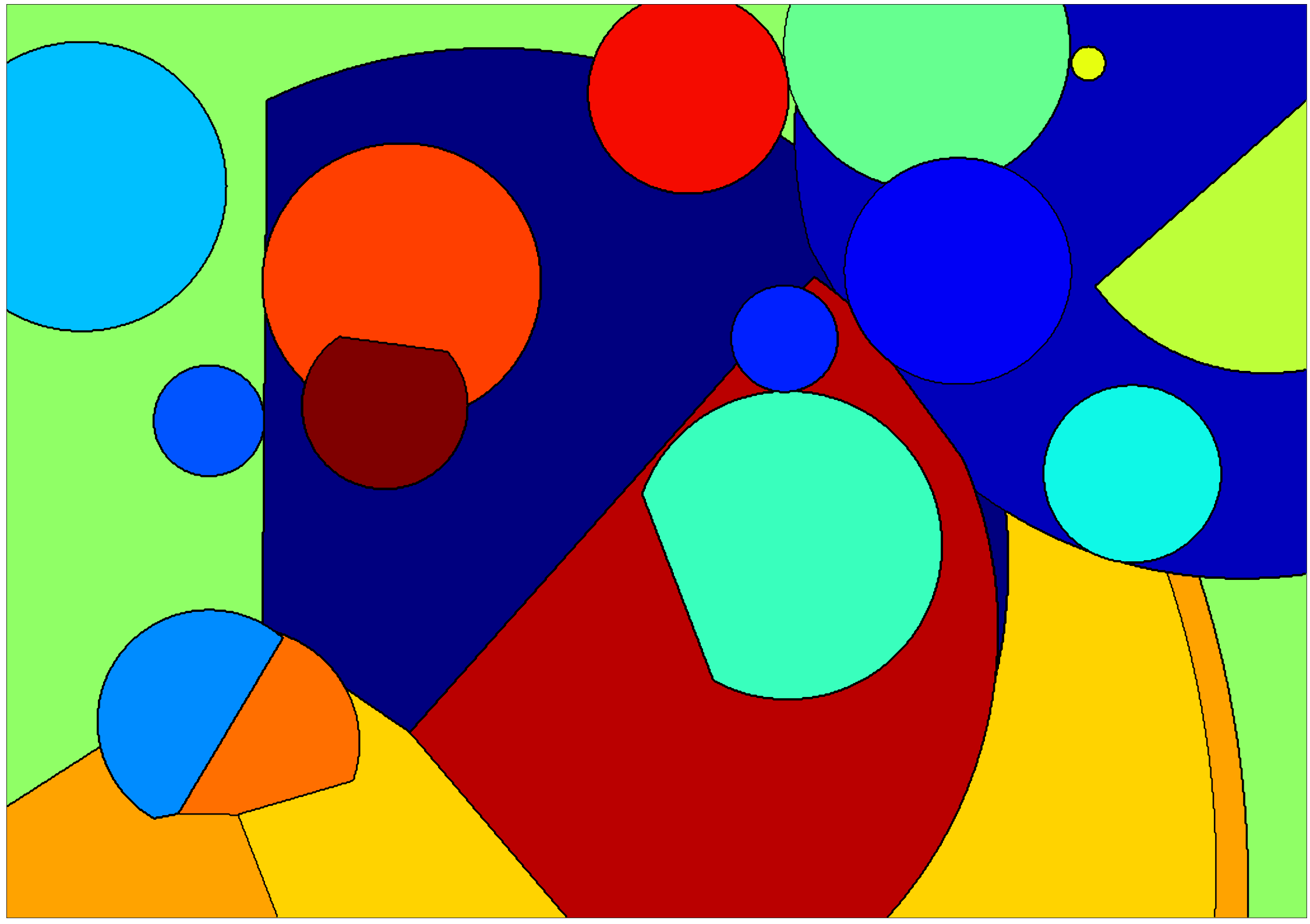
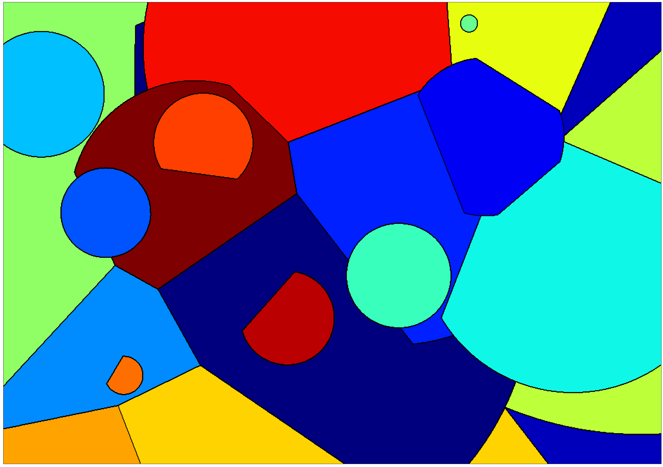
Provisioning
Provisioning tells how much of the required pixels the sites can handles. Underprovisioning will create holes in the partition as the sites shrink down to balls centered around the centers.
[11]:
smup.compute(provisioning=.6, seed=42)
smup.display()
[12]:
smup.compute(provisioning=.2, seed=42)
smup.display()
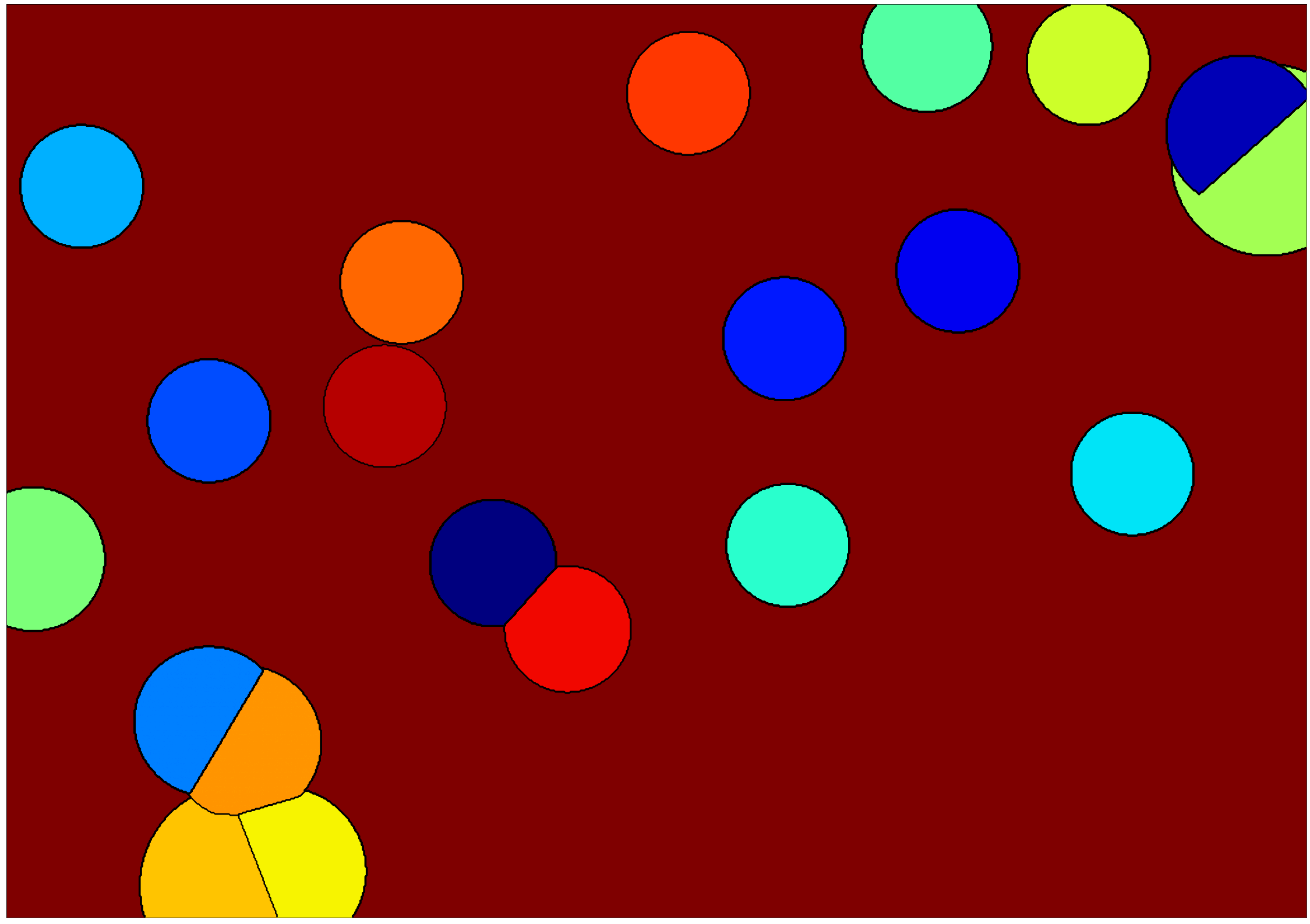
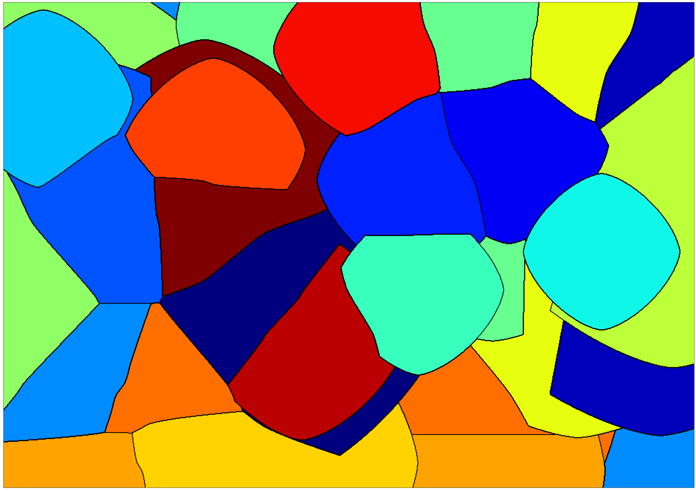
On the other hand, overprovisioning will allow to reach the Voronoi diagram. Because yep, you can see a Voronoi diagram as a special case of stable-matching!
[13]:
smup.compute(provisioning=1.2, seed=42)
smup.display()
[14]:
smup.compute(provisioning=6, seed=42)
smup.display()
Heterogeneous areas
Instead of having the same area for all sites, diversity can be enabled.
[15]:
smup.compute(heterogeneous_areas=True, seed=42)
smup.display()
[16]:
smup.compute(heterogeneous_areas=True, provisioning=1.3, seed=42)
smup.display()
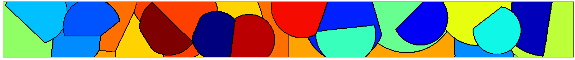
Size
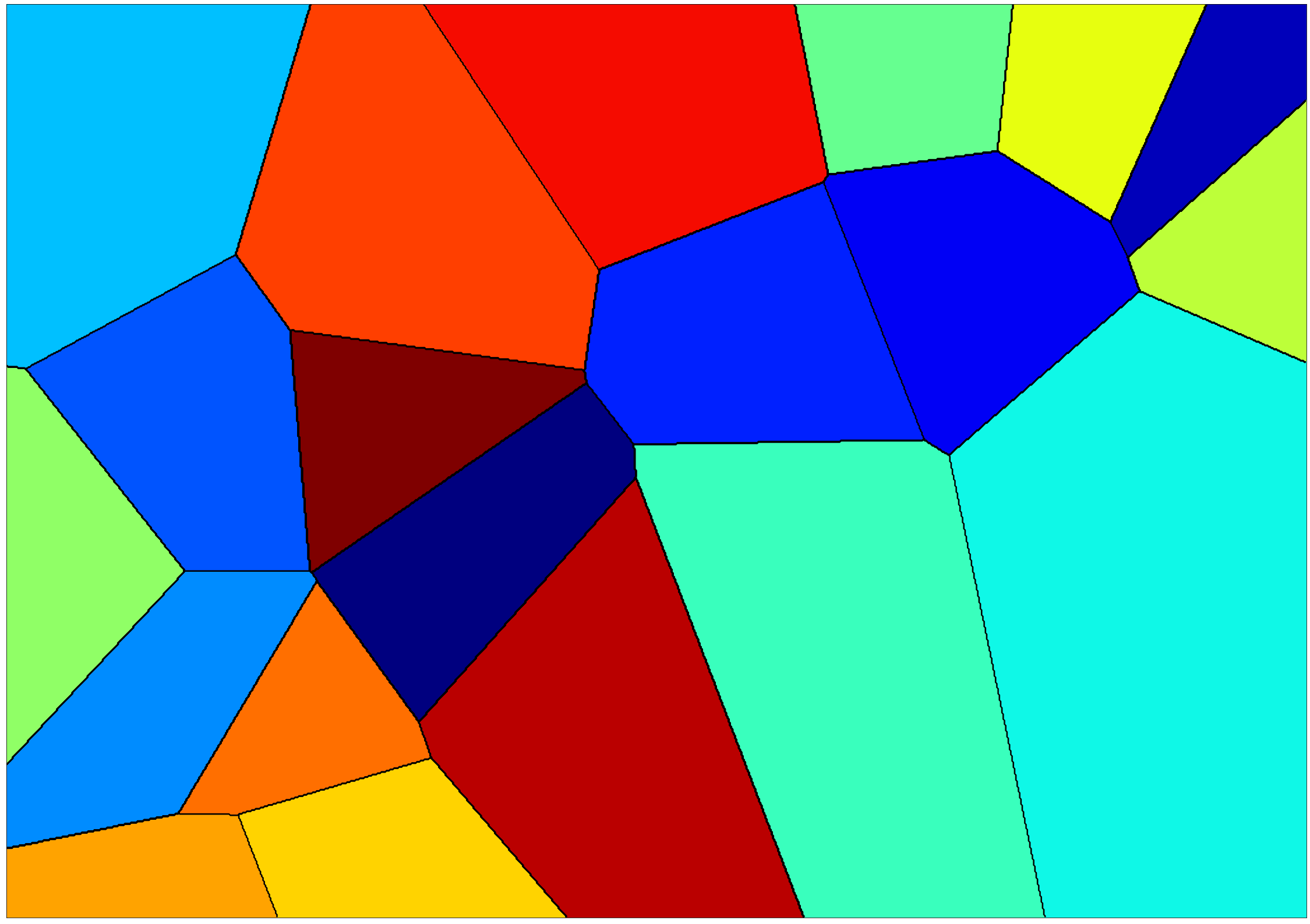
With x and y you can change the size of the picture. Note that the computational time is \(\tilde{O}(xys)\) and the memory occupation is \(O(xys)\). The following draws a fast rough version of the picture above.
[17]:
smup.compute(x=100, y=72, norm='inf', seed=42)
smup.display()
You can use x or y to change the aspect ratio, for example if you want to produce a banner.
[18]:
smup.compute(y=100, seed=42)
smup.display()
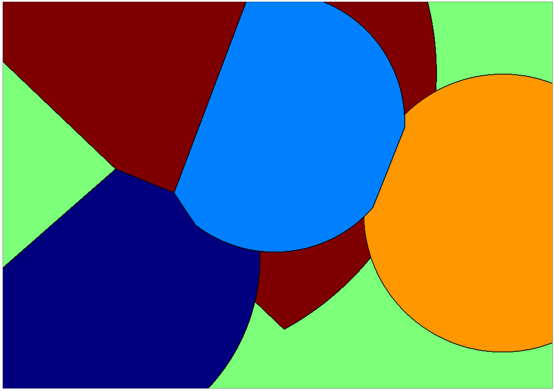
Number of areas
Less sites will give you a simple smup.
[19]:
smup.compute(s=5)
smup.display()
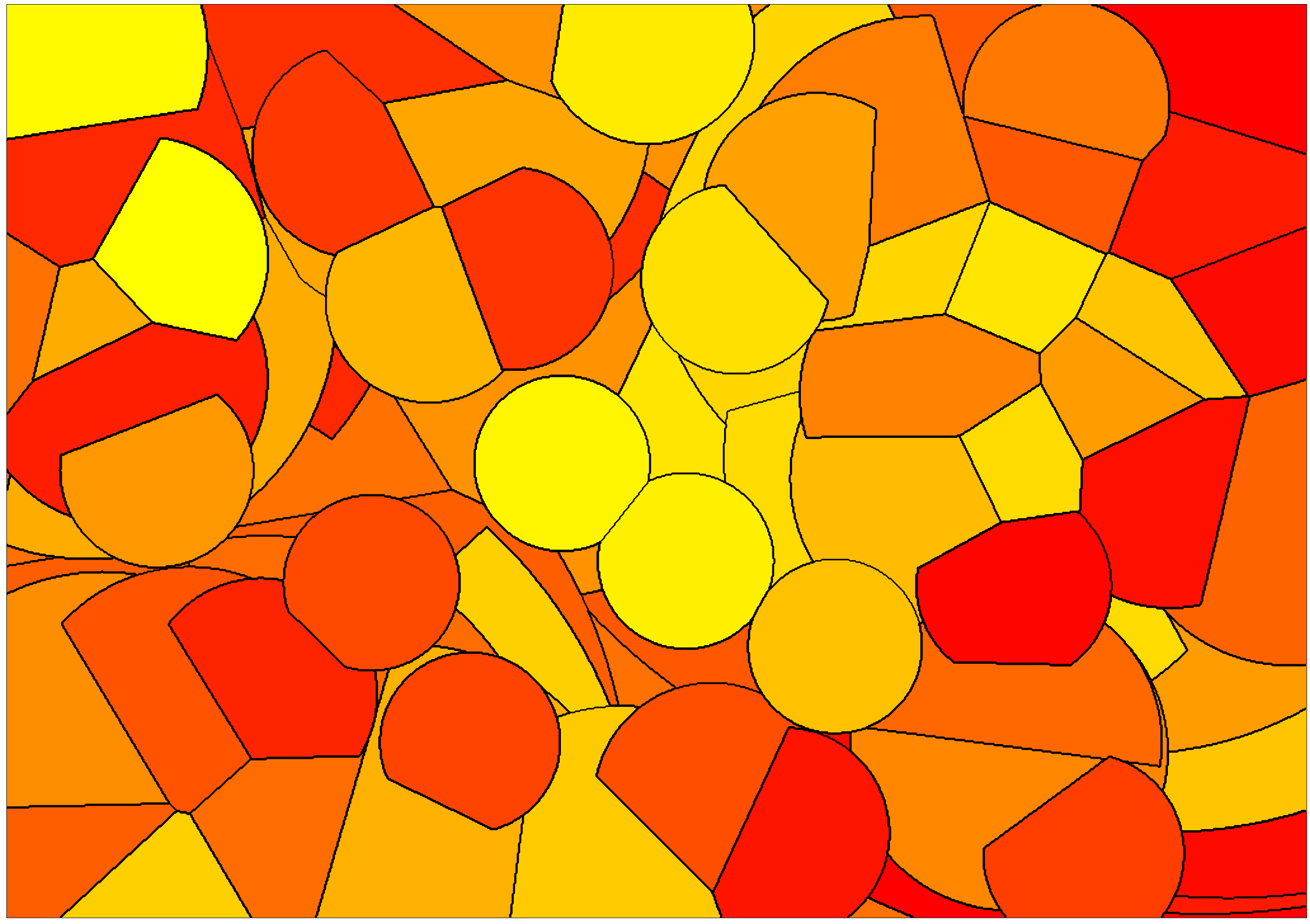
More sites will produce a richer smup. Beware of time and space complexities that grow with s.
[20]:
smup.compute(s=50)
smup.display()

Display parameters
Colormap
You can use any Matplotlib maps to change the colors of your smup. See the list here: https://matplotlib.org/stable/tutorials/colors/colormaps.html
[21]:
smup.display(cmap="spring")

[22]:
smup.display(cmap="autumn")
[23]:
smup.display(cmap="hsv")
Centers
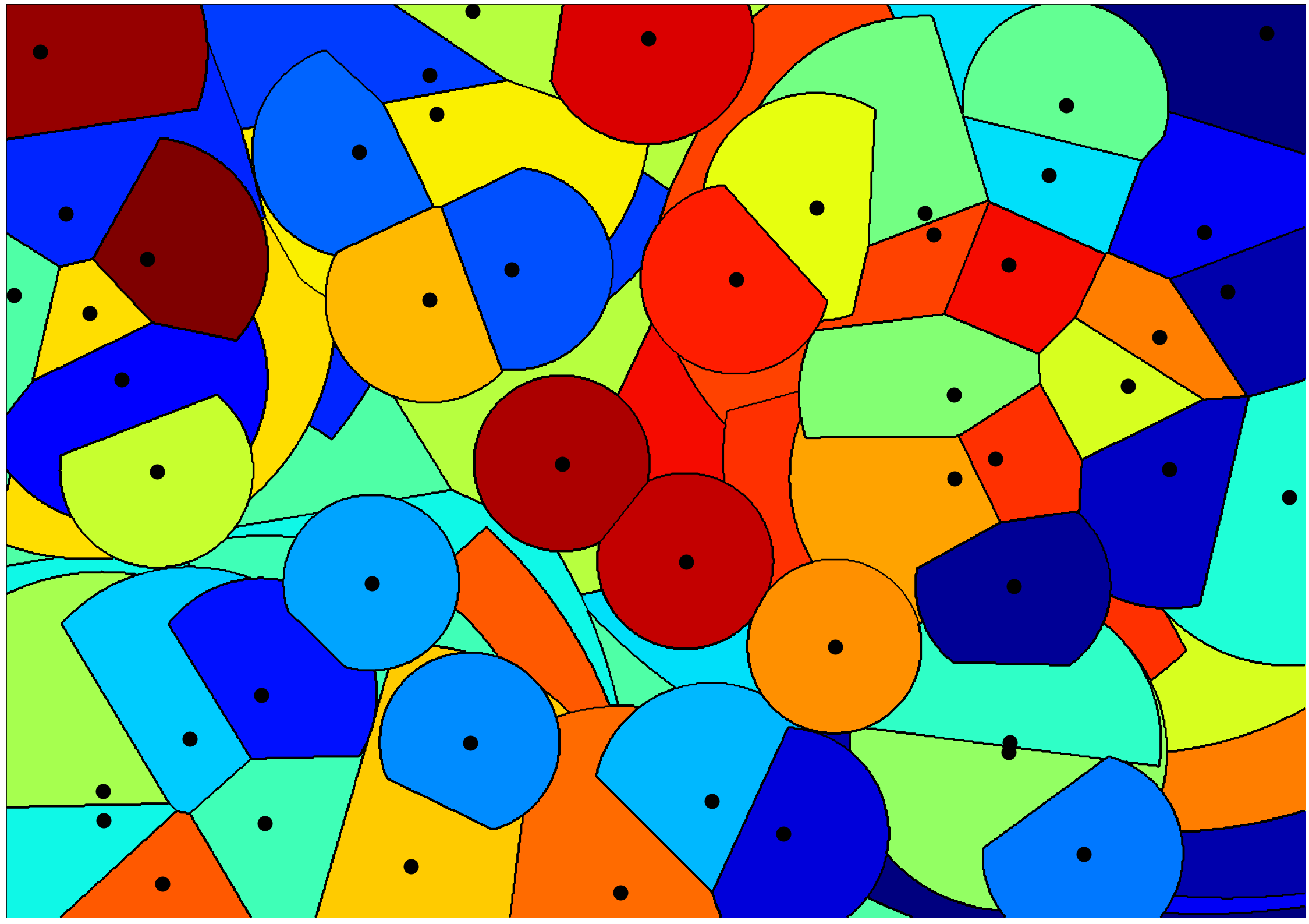
The site centers help to understand the mechanisms of a smup. Removes a bit of the mystery, but you can show them if you want.
[24]:
smup.display(draw_centers=True)

On the other hand, if you wish to show big centers, you can!
[25]:
smup.display(draw_centers=True, center_size=50)
Saving
To save the picture, just feed the save parameter with filename. Cf https://balouf.github.io/smup/reference/index.html#smup.smup.Smup.display
Theory
A smup is just a \(b\)-matching between a set of centers drawn at random and the pixels of the picture, with distances used as preferences. Funny thing with distance-based preferences is that they tend to follow a power-law distribution, which means that while most of the pixels will be attached close to their center, some pixels are exiled far away, possibly to the other end of the picture. Another funny thing is that if you run the propose/dispose algorithm by increasing distance, there is no rejection after acceptance, which allows to speed up the algorithm a bit.
The paragraph above doesn’t mean anything to you? Don’t panic, here are a few pointers:
College Admissions and the Stability of Marriage, the original article on stable matchings.
A Stable Marriage of Poisson and Lebesgue, a mathematical approach to smups.
The Stable Configuration of Acyclic Preference-Based Systems, my own (useless?) research on the topic.