Simulations

A significant part of the Stochastic Matching package is devoted to simulations, allowing to check the practical value of theoretical results and to explore new conjectures.

Note

The refresh parameter below tells if the simulation should run if a simulation file already exists. It is there to modify this notebook without re-running all simulations.

refresh = False

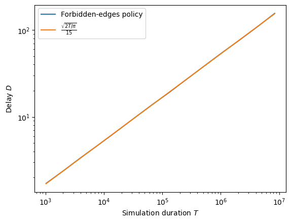
Drift of optimal solution for injective-only vertices

Injective-only vertices have the property that any regret-optimal policy, like forbidden-edges, must generate the delay of an unbiased random walk, which is of the order of \(\sqrt(T)\).

We can verify that on an injective-only vertex of the diamond graph.

import stochastic_matching as sm
diamond = sm.CycleChain()
rewards = [0, 1, 1, 1, 0]
diamond.show_flow(flow=diamond.optimize_rates(rewards))

Reload

Let us build iterated experiments to measure the delay as a function of the simulation time \(T\).

from stochastic_matching import XP, Iterator, evaluate
from multiprocess import Pool

xp  = XP(name='RW', simulator='longest', model=sm.CycleChain(),
         iterator=Iterator('n_steps', [2**t for _ in range(10000) for t in range(10, 24)], name='T'),
         max_queue=10000,
         forbidden_edges=True, rewards=[0, 1, 1, 1, 0])

Note

• An XP is designed by specifying static and varying parameters. Here we fix a ML policy with forbidden edges that aims for an injective-only vertex of the diamond graph, with extra queue capacity to absorb instability, and varying simulation duration.

• Most scenarios involve stable policies, so one very long simulation is enough. Here, we focus on the short-term to mid-term performance of an unstable policy, so redundancy is required. We choose 10,000.

• In its low level implementation, the package allows to stop/restart a simulation. That means that we could just run long-term simulations and monitor the state at some stopping points. We don’t do that here for simplicity. As a result, we know that the proposed experiment is could be sped up by a factor 2 at the price of extra XP design.

• The individual simulations are ordered like abcdabcdabcd... instead of aaabbbcccddd... to ease the parallelism.

OK, let’s run 140,000 simulations of duration up from \(1024\) to \(2^{23}\approx 8.10^6\) time steps. Count a bit more than 2 sims per second and per logical core on 2+Ghz computers, in average.

with Pool() as p:
    res = evaluate(xp, ["delay"], p, cache_name="drift", cache_overwrite=refresh)

Let’s gather everything.

from collections import defaultdict
import numpy as np

metrics = defaultdict(list)
for t, d in zip(res['RW']['T'], res['RW']['delay']):
    metrics[t].append(d)
for k, v in metrics.items():
    metrics[k] = np.average(v)
steps = [k for k in metrics]
delay = [v for v in metrics.values()]

And… plot the results!

from matplotlib import pyplot as plt
plt.loglog(steps, delay, label='Forbidden-edges policy')
plt.loglog(steps, [np.sqrt(2*t/3.14)/15 for t in steps], label='$\\frac{\\sqrt{2T/\\pi}}{15}$')
plt.xlabel('Simulation duration $T$')
plt.ylabel('Delay $D$')
plt.legend()
plt.show()

Vertices of simple graphs

Our objective here is to evaluate the performance of policies that try to achieve a given vertex of the polytope of a matching problem \((G, \lambda)\), starting with the assumption that \(G\) is a simple graph.

Important

In our framework, polytopes are always embedded in the space of matching rates, so a vertex represents a matching rate. For simplicity, we also identify a vertex with its positive support, meaning the set of edges where the matching rate is positive, which can be viewed as a subgraph of \(G\).

Preparation

First, some settings that should apply to all our simulations.

n_steps = 10**10
common = {
        "n_steps": n_steps,
        "max_queue": 50000,
        "seed": 42,
}

Then, we write a small mixer of common and specific parameters.

def xp_builder(common, specific):
    return sum([XP(name=k, **common, **v) for k, v in specific.items()])

We prepare specific parameters for each policy.

from numba import njit

k_range = Iterator("k", [2**i for i in range(14)])
e_range = Iterator("epsilon", np.logspace(-3, 0, 10), name="ϵ")
b_range = Iterator("beta", np.logspace(-3, 1, 10), name="β")
def exp_fad(x):
    return njit(lambda t: (t+1)**x)
v_range = Iterator("fading", [exp_fad(x) for x in np.linspace(0., 1., 10)], name="V")

specific = {
    'k-filtering': {'simulator': "longest", 'forbidden_edges': True,
                    'iterator': k_range},
    'EGPD': {'simulator': "virtual_queue",
             'iterator': b_range},
    "ϵ-filtering": {'simulator': "e_filtering",
                    'iterator': e_range},
    "EGPD+": {'simulator': "virtual_queue", 'alt_rewards': 'gentle',
              'iterator':  b_range},
    "CRPD": {'simulator': 'constant_regret',
             'iterator': v_range},
    "Taboo": {'simulator': 'longest', 'forbidden_edges': True}
           }

Finally, a display function with a few options.

name_relabelling = {'Taboo': '$\\Phi_{E^*}$'}
def display_res(res, view="loglog", x_max=None, y_min=10**-8, y_max=None):
    if view == "loglog":
        plot = plt.loglog
    elif view == "logx":
        plot = plt.semilogx
    else:
        raise ValueError(f"{view} is not a recognized display view.")
    names = [k for k in res]
    colors = {k: v for k, v in zip(names,
                                   plt.rcParams['axes.prop_cycle'].by_key()['color'])}
    for k in sorted(names, key=lambda k: -np.average(res[k]['regret'])):
        v = res[k]
        name = name_relabelling.get(k, k)
        delay, regret = np.array(v["delay"]), np.array(v["regret"])
        if isinstance(v["delay"], list):
            mask = delay > 0
            plot(np.abs(delay[mask]), np.abs(regret[mask]), marker="o",
                 label=name, color=colors[k])
        else:
            if y_max is None:
                plot([delay], [regret], marker="o", label=name, color=colors[k])
            else:
                plot([delay, delay], [y_min, y_max], '--', label=name, color=colors[k])

    plt.ylabel("Regret")
    plt.xlabel("Delay")
    if view == "logx":
        plt.ylim([0, None])
    plt.xlim([None, x_max])
    if y_max:
        plt.ylim([y_min, y_max])
    plt.legend()
    plt.show()

We are now ready to start various experiments.

Diamond

Injective-only vertex

Let’s reach an injective-only vertex.

import stochastic_matching as sm
diamond = sm.CycleChain()
rewards = [1, 2.9, 1, -1, 1]
diamond.show_flow(flow=diamond.optimize_rates(rewards))

Reload

Note

The rewards are adversarial here: the largest reward corresponds to a taboo edge.

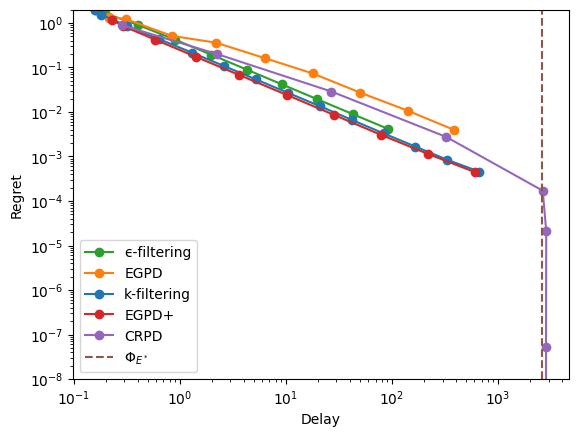
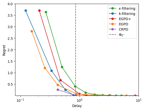
Let us compute the delay/regret trade-offs and display the results.

xps = xp_builder({'model': diamond, 'rewards': rewards, **common}, specific)
with Pool() as p:
    res = evaluate(xps, pool=p, cache_name="diamond-injective",
                   cache_overwrite=refresh)
display_res(res, y_max=.4)

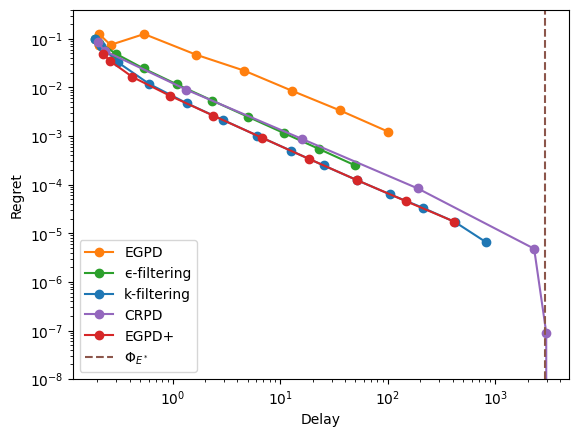
Important

A simulation can only provide a finite-horizon estimate of the long-term behavior of a policy. In particular, it will always yield a finite delay even for policies that are proven to be unstable, i.e. those that have infinite long-term delay.

This explains why some of the policies considered here seem to achieve finite delay and zero rate-regret (that is, constant global-regret) in simulations.

For injective-only vertices, unstability stems from arrival deviations that behave roughly like an unbiased random walk, with magnitude on the order of \(\sqrt(T)\), where \(T\) is the number of time steps simulated (cf the first serie of experiments above). If \(\sqrt(T)\) is small relative to the typical long-term delay of a policy (which is always the case for unstable policies), the trade-off between regret and delay cannot be observed through simulations.

As a consequence, for injective-only vertices:

• The regret values observed in the far right portion of the figures should be ignored, as they reflect discrepancies between long-term and finite-horizon values.

• Simulations should be run over as many time steps as possible to broaden the parameter range over which long-term and finite-horizon estimates coincide.

Take-away:

• EGPD has not a good trade-off;

• \(\epsilon\)-filtering and CRPD have average performance;

• \(k\)-filtering and EGPD+ are the best here.

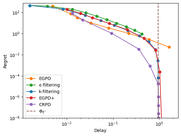
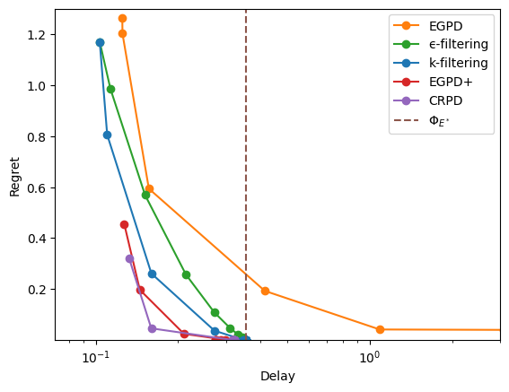
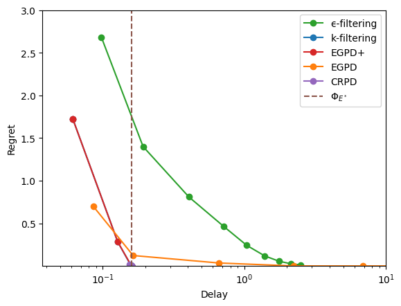
Bijective vertex

We now change the rates and rewards so that the target is a bijective vertex.

diamond.rates = [4, 4, 4, 2]
rewards = [-1, 1, 1, 1, 2.9]
diamond.show_flow(flow=diamond.optimize_rates(rewards))

Reload

Note

The rewards are even more adversarial here: the largest reward corresponds the unique taboo edge, while a live edge has a negative reward.

As before, let’s see the trade-offs.

xps = xp_builder({'model': diamond, 'rewards': rewards, **common}, specific)
with Pool() as p:
    res = evaluate(xps, pool=p, cache_name="diamond-bijective",
                   cache_overwrite=refresh)
display_res(res, view="logx", x_max=1, y_max=.15)

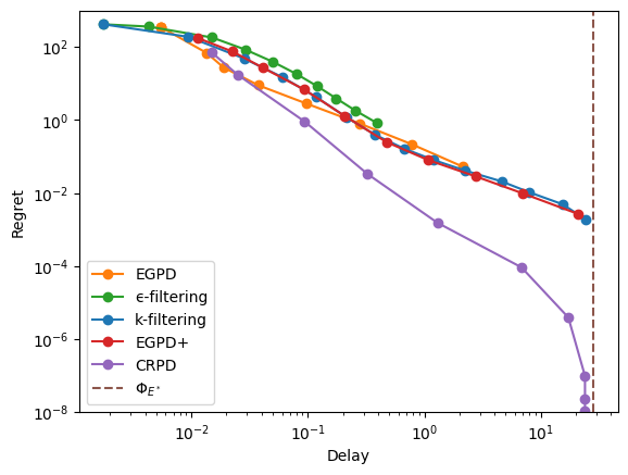
Codomino

Injective-only vertex

codomino = sm.Codomino(rates=[2, 4, 2, 2, 4, 2])
rewards = [-1, 1, -1, 1, 4.9, 4.9, 1, -1]
codomino.show_flow(flow=codomino.optimize_rates(rewards))

Reload

xps = xp_builder({'model': codomino, 'rewards': rewards, **common}, specific)
with Pool() as p:
    res = evaluate(xps, pool=p, cache_name="codomino-injective",
                   cache_overwrite=refresh)
display_res(res, y_max=2 )

Bijective-only vertex

Here, we choose rewards so that all taboo edge have a positive weight, while two live edges have a negative weight.

codomino.rates = [4, 5, 5, 3, 3, 2]
rewards = [3.1, -1, 1,  1, -1, 0,  1, 0]
codomino.show_flow(flow=codomino.optimize_rates(rewards))

Reload

xps = xp_builder({'model': codomino, 'rewards': rewards, **common}, specific)
with Pool() as p:
    res = evaluate(xps, pool=p, cache_name="codomino-bijective",
                   cache_overwrite=refresh)
display_res(res, view='logx', x_max=3, y_max=1.3)

Larger graphs

n, d = 100, 20
er = sm.ErdosRenyi(n=n, d=d, seed=42)
er.m

1006

To select a vertex, we draw random rewards, which are optimized at a unique point w.h.p.

rewards = np.random.rand(er.m)

Injective-only vertex

vertex = er.optimize_rates(rewards)
np.sum(vertex>0)

np.int64(97)

xps = xp_builder({'model': er, 'rewards': rewards, **common}, specific)
with Pool() as p:
    res = evaluate(xps, pool=p, cache_name="er-injective",
                   cache_overwrite=refresh)
display_res(res, y_max=1000)

Bijective vertex

np.random.seed(42)
er.rates = er.rates + 5*np.random.rand(n)
vertex = er.optimize_rates(rewards)
np.sum(vertex>0)

np.int64(100)

xps = xp_builder({'model': er, 'rewards': rewards, **common}, specific)
with Pool() as p:
    res = evaluate(xps, pool=p, cache_name="er-bijective",
                   cache_overwrite=refresh)
display_res(res, y_max=800)

Vertices of hypergraphs

We now remove the hypothesis that \(G\) is a simple graph. We need to adjust some policy settings accordingly, switching from longest queue to virtual queue to ensure stability.

for k in ['k-filtering', 'Taboo']:
    specific[k]['simulator'] = 'virtual_queue'
    specific[k]['alt_rewards'] = 'gentle'
specific['ϵ-filtering']['base_policy'] = 'virtual_queue'

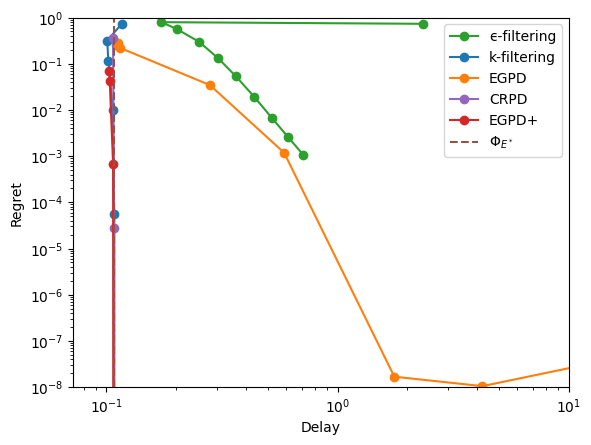
Abandonment

To start, we consider a diamond graph where one item class can be abandonned and where the optional solution is to abandon it entirely. As usual, we pick adversarial rewards so that the resulting vertex looks a bit counter-intuitive.

# Add a self-loop to the last node of a diamond.
incidence = np.hstack([diamond.incidence, np.array([[0, 0, 0, 1]]).T])
# Create model
modified_diamond = sm.Model(incidence=incidence, rates=[4, 4, 4, 2])
# Set rewards
rewards = [-1, 1, 1, 1, 3, 2]
# Show optimal rates
modified_diamond.show_flow(flow=modified_diamond.optimize_rates(rewards))

Reload

xps = xp_builder({'model': modified_diamond, 'rewards': rewards, **common}, specific)
with Pool() as p:
    res = evaluate(xps, pool=p, cache_name="abandonment",
                   cache_overwrite=refresh)
display_res(res, x_max=10, y_max=1)

Nazari & Stolyar example

See https://arxiv.org/abs/1608.01646 for details.

First arrival rates

ns19 = sm.NS19(rates=[1.2, 1.5, 2, 0.8])
rewards = [-1, -1, 1, 2, 5, 4, 7]
ns19.show_flow(flow=ns19.optimize_rates(rewards))

Reload

xps = xp_builder({'model': ns19, 'rewards': rewards, **common}, specific)
with Pool() as p:
    res = evaluate(xps, pool=p, cache_name="ns19-a", cache_overwrite=refresh)
display_res(res, view='logx', x_max=10, y_max=4)

Second arrival rates

ns19.rates = [1.8, .8, 1.4, 1]
ns19.show_flow(flow=ns19.optimize_rates(rewards))

Reload

Important

In the example above, the first self-edge is used despite having a negative reward: it is an example of a graph with self-edges where the optimal stable solution is not the same than the optimal solution.

Note that the optimal solution can always be made stable (if \(G\) is surjective) by adding zero-reward mono-edges.

xps = xp_builder({'model': ns19, 'rewards': rewards, **common}, specific)
with Pool() as p:
    res = evaluate(xps, pool=p, cache_name="ns19-b", cache_overwrite=refresh)

display_res(res, view='logx', x_max=10, y_max=3)

Flexibility of greedy policies

Complete graph

For complete graphs, all greedy policies are equivalent because there is never any true choice to make in that case. Let us check that by running a few greedy policies.

We will use the graph \(K_4\), which has a 2-D kernel. With uniform arrival rates, its polytope is a triangle.

complete = sm.Complete(n=4)
complete.vertices

[{'kernel_coordinates': array([-1., -1.]),
  'edge_coordinates': array([0., 0., 3., 3., 0., 0.]),
  'null_edges': [0, 1, 4, 5],
  'bijective': False},
 {'kernel_coordinates': array([-1.,  2.]),
  'edge_coordinates': array([3., 0., 0., 0., 0., 3.]),
  'null_edges': [1, 2, 3, 4],
  'bijective': False},
 {'kernel_coordinates': array([ 2., -1.]),
  'edge_coordinates': array([0., 3., 0., 0., 3., 0.]),
  'null_edges': [0, 2, 3, 5],
  'bijective': False}]

For the comparison, we will consider the following greedy policies:

complete_policies = {
    "Longest": {"simulator": "longest"},
    "FCFM": {"simulator": "fcfm"},
    "Random Edge": {"simulator": "random_edge"},
    "Random Item": {"simulator": "random_item"},
    "Priority": {"simulator": "priority", "weights": [1, 10, 0, -1, 3, 4]},
}

We run the simulation, gathering the resulting matching rate in edge and kernel coordinates:

def flow_kernel_coordinates(simu):
    flow = simu.flow
    return simu.model.edge_to_kernel(flow)
xps = xp_builder({'model': complete, **common}, complete_policies)
with Pool(5) as p:
    res = evaluate(
        xps, ["flow", flow_kernel_coordinates], pool=p, cache_name="complete",
        cache_overwrite=refresh
    )
res

{'Longest': {'flow': array([1.00000059, 1.0000066 , 1.00001283, 1.0000111 , 1.00000862,
         0.99996026]),
  'flow_kernel_coordinates': array([0., 0.])},
 'FCFM': {'flow': array([1.00000059, 1.0000066 , 1.00001283, 1.0000111 , 1.00000862,
         0.99996026]),
  'flow_kernel_coordinates': array([0., 0.])},
 'Random Edge': {'flow': array([1.00003558, 1.00002742, 0.99995652, 0.99996954, 0.99997213,
         1.00003881]),
  'flow_kernel_coordinates': array([0., 0.])},
 'Random Item': {'flow': array([1.00003558, 1.00002742, 0.99995652, 0.99996954, 0.99997213,
         1.00003881]),
  'flow_kernel_coordinates': array([0., 0.])},
 'Priority': {'flow': array([1.00000059, 1.0000066 , 1.00001283, 1.0000111 , 1.00000862,
         0.99996026]),
  'flow_kernel_coordinates': array([0., 0.])}}

Tip

In the results above, the randomized policies (on Items and Edges) have not exactly the same rate than the deterministic policies, despite the use of a seed. The reason is that there is one unique random generator per simulator, so having a randomized policy impacts the drawing of arrivals (even if the number of possibilities is always reduced to 1).

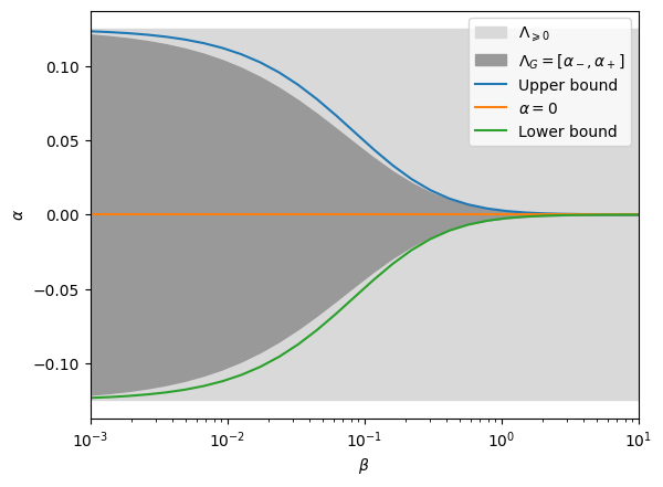
Diamond

For the diamond, the capacity of greedy policies to affect the matching rates depends on the traffic \(\beta\) on the central edge, which corresponds to the unbalance between the two opposite pairs of nodes. Roughly speaking, when the central traffic is scarse, greedy policies get to choose more, leading to a greater influence.

First, let us build the experiments for various \(\beta\). Note that all models are symmetric so we can focus on targeting one vertex.

def beta_to_model(beta):
    return sm.CycleChain(
        names=[str(i) for i in range(1, 5)],
        rates=[1 / 4, 1 / 4 + beta, 1 / 4 + beta, 1 / 4],
    )

n_points = 30
β_vect = np.logspace(-3, 1, n_points)
model_iter = Iterator("model", β_vect, "β", beta_to_model)

xps = XP("Greedy vertex", simulator="priority", weights=[1, 0, 0, 0, 1], iterator=model_iter, **common)

What we want to measure are the kernel coordinate \(\alpha\) of the matching rates of the policy.

def alpha(simu):
    flow = simu.flow
    return (flow[0] + flow[-1] - flow[1] - flow[3]) / 4

with Pool() as p:
    res = evaluate(xps, alpha, pool=p, cache_name="greedy-diamond", cache_overwrite=refresh)
res = np.array(res["Greedy vertex"]["alpha"])

Theoretical bounds:

def min_flow2(beta):
    q13 = 1 / (4 * beta)
    q2 = 1 / 2 + 2 * beta
    p0 = 1 / (1 + q13 + 2 * q2)
    return p0 * q2 / 4 + p0 / (1 + 8 * beta) * (1 / 4 + beta) - 1 / 8


lbi = [min_flow2(β) for β in β_vect]
ubi = [-min_flow2(β) for β in β_vect]

Results:

plt.fill_between(
    β_vect,
    -1 / 8 * np.ones(n_points),
    1 / 8 * np.ones(n_points),
    label="$\\Lambda_{\\geqslant 0}$",
    color=[0.85, 0.85, 0.85, 1],
)
plt.fill_between(
    β_vect,
    -res,
    res,
    label="$\\Lambda_G = [\\alpha_-, \\alpha_+]$",
    color=[0.6, 0.6, 0.6, 1],
)

plt.semilogx(β_vect, ubi, label="Upper bound")
plt.semilogx(β_vect, np.zeros(n_points), label="$\\alpha=0$")
plt.semilogx(β_vect, lbi, label="Lower bound")

plt.xlabel("$\\beta$")
plt.ylabel("$\\alpha$")
plt.legend()
plt.xlim([β_vect[0], β_vect[-1]])
plt.show()

Fish graph

The Fish graph, with properly designed arrival rates, is a counter-example to the lack of flexibility of greedy policies in surjective-only graphs, as it is feasible for a family of greedy policies to converge to the vertex. There, however, a price to pay in terms of delay, despite the fact that the vertex is bijective.

Here is the graph:

fish = sm.KayakPaddle(
    3, 0, 4, names=[str(i) for i in range(1, 7)], rates=[4, 4, 3, 2, 3, 2]
)
fish.show_kernel(disp_rates=False, disp_flow=True)

Reload

Our target is the bijective vertex \(\alpha=1/2\).

fish.show_flow(disp_rates=False, flow=fish.kernel_to_edge([1/2]))

Reload

Rate limitation lemma

To build the policy, the first part consists in noticing that if nodes 3 is forced to prioritize the tail of the fish (nodes 1 and 2), then the rate that 3 can send to the body is at most \(9/11\approx 0.818\). This result does not depend on the body shape so we heck it on a simple frying pan (the body reduced to one node outside of 3).

paw = sm.Tadpole(names=[str(i) for i in range(1, 5)], rates=[4, 4, 3, 1])
paw.stabilizable

True

paw.base_flow

array([3., 1., 1., 1.])

paw.run("priority", weights=[0, 1, 1, 0], max_queue=10**7, n_steps=10**7)

True

paw.show_flow(disp_rates=False)

Reload

Unstable greedy policy lemma

Building on the rate limitation, one can craft an instable greedy policy that starves the body of the fish. Starvation induces a constantly growing number of waiting items. Using priorities, we can shape the policy so that waiting items are mostly of type 4. As a side-effect, that would nullify the edge \((3, 6)\), which is what we want.

fish.run("priority", weights=[0, 3, 3, 2, 0, 0, 2], max_queue=10**7, n_steps=10**7, seed=42)
fish.show_flow(disp_rates=False)

Reload

We can check that the queue is concentrated on node 4.

fish.simulator.avg_queues

array([8.51466300e-01, 8.47361100e-01, 2.00000000e-07, 5.01960123e+04,
       3.00000000e-07, 1.98790250e+00])

To finalize, all what we need is relax the unstable greedy policy into a stable policy when queues are too high.

fish.run(
    "priority",
    weights=[0, 3, 3, 2, 0, 0, 2],
    threshold=100,
    counterweights=[0, 1, 1, 2, 0, 0, 2],
    n_steps=10**7,
    seed=42
)
fish.show_flow(disp_rates=False)

Reload

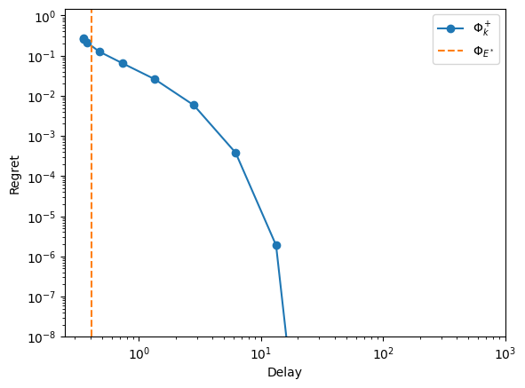
Evaluation

As often, we have a delay/regret trade-off.

rewards = [2, 2, 2, 1, -1, 0, 1]
t_range = Iterator("threshold", 2 ** (np.arange(14)), "k")
name = '$\\Phi_k^+$'
fish_policies = {name: {'simulator': 'priority', 'weights': [0, 3, 3, 2, 0, 0, 2],
                                'counterweights': [0, 1, 1, 2, 0, 0, 2], 'iterator': t_range},
                 'Taboo': specific['Taboo']}

Note

The priority policy has no built-in regret management, so we need to post-compute it.

fish.simulator = None
xps = xp_builder({'model': fish, **common}, fish_policies)
with Pool() as p:
    res = evaluate(xps, pool=p, metrics=["delay", "regret", "flow"], cache_name="fish",
                   cache_overwrite=refresh)

def regret(model, flow, rewards):
    original_rates = model.rates
    model.rates = model.incidence @ flow
    best_flow = model.optimize_rates(rewards)
    model.rates = original_rates
    return rewards @ (best_flow - flow)

res[name]['regret'] = [regret(fish, flow, rewards) for flow in res[name]['flow']]

display_res(res, x_max=1000, y_max=1.5)