Using Smart Cruise

This tutorial demonstrates how to use smart-cruise to find Pareto-optimal trajectories.

Note on Generality: While this example uses liner-style parameters, the underlying model is completely generic. It applies to any vehicle with state-dependent energy consumption: UAVs, AUVs (underwater vehicles), ground vehicles, ships, etc. See the main documentation for more details on adapting the model to other domains.

SC finds the Pareto front of energy/time optimal trajectories.

• Distance, height, and speeds are discrete. Finer granularity leads to better solutions.

• Speed is governed by a backoff parameter that tells when the vehicle can adjust speed.

• Energy (“weight”) and time budgets are continuous.

• The default cost model is randomized, taking into account position, height, speed, remaining energy, and height change.

• For each internal state (distance, height, speed, backoff), a Pareto front is computed. The front is quantized for a trade-off between computation speed and solution quality.

In this tutorial notebook, we will investigate the impact of Pareto quantization on three scenario, then have a look at the best trajectories for the last scenario.

Preparation

We will use Joblib to parallelize simulations with various quantization on a given scenario.

Note

This tutorial uses joblib for parallelization. You can install it with:

pip install joblib

The following cell chews all the work for us. It computes Pareto-optimal trajectories with various internal front quantizations.

from functools import partial

from joblib import Parallel, delayed

from smart_cruise import CostRandom, Cruise

pms = [2**i for i in range(7)][::-1]
n_s = 31


def traj_maker(pm, w0, t0):
    model = CostRandom(seed=42, n_s=n_s)
    cruise = Cruise(model)
    cruise.parameters.pareto_max = pm
    cruise.compute(w0=w0, t0=t0)
    return pm, cruise.trajectories


def pms_trajs(w0, t0):
    return Parallel(n_jobs=-1)(delayed(partial(traj_maker, w0=w0, t0=t0))(pm) for pm in pms)

Tight budget

Let us start with a tight scenario (low weight and time budget):

res = pms_trajs(w0=21800.0, t0=21800.0)

Let’s write a function to display the various results:

from matplotlib import pyplot as plt


def show_pareto(res, wmin=0, tmin=0, file=None):
    for pm, traj in res:
        if traj.trajs is None:
            continue
        w, t = traj.get_front()
        plt.plot(w, t, label=f"$S={pm}$")
    plt.xlabel("Remaining energy")
    plt.ylabel("Spare time")
    plt.xlim([wmin, None])
    plt.ylim([tmin, None])
    plt.legend()
    plt.show()

Let’s look at the result!

show_pareto(res)

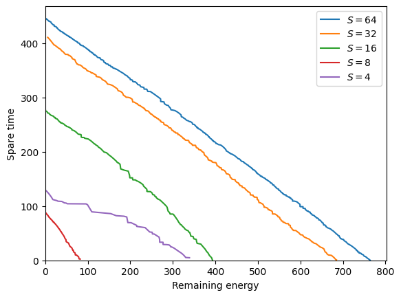
• The scenario is so tight that only a few bad decisions make it impossible to find a viable path.

• In other words: if the sampling size \(S\) is too low we cannot find solutions.

• For intermediate values of \(S\), monotonicity is not guaranteed (there is a chance factor).

• Starting from 16, we have solutions. Their quality increases with the number of samples kept.

Bigger budget

Now look at a scenario with overkill budget:

res = pms_trajs(w0=32000.0, t0=32000.0)

Let’s look at the result!

show_pareto(res, wmin=4000, tmin=2000)

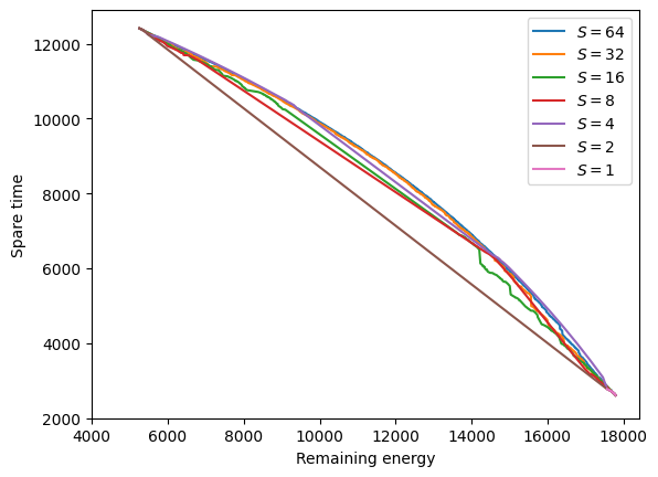
• Here all choices lead to a viable path.

• Strong quantization (\(S\leq 16\)) finds solutions but with poor quality.

• Low quantization seems to converge to the optimal Pareto front.

Note

The tight scenario we just saw can be interpreted as a zoom of the bigger budget on an area that preserves some fixed quantities of the resources. More precisely, if we zoom to keep \(32000-21800 = 10200\), we get the tight budget.

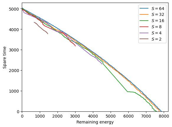
Middle budget

res = pms_trajs(w0=25000.0, t0=25000.0)

Let’s look at the result!

show_pareto(res)

Let’s look at the result!

Trajectories

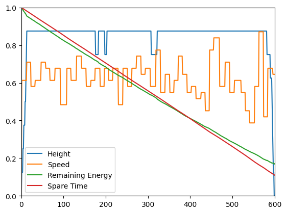
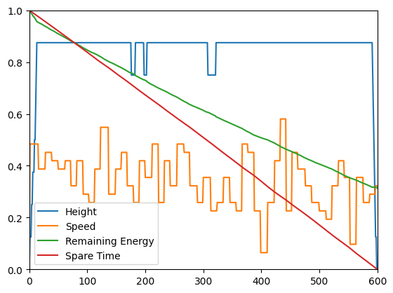
Best weight preserving trajectory:

_, trajs = res[0]
trajs.plot_traj(0)

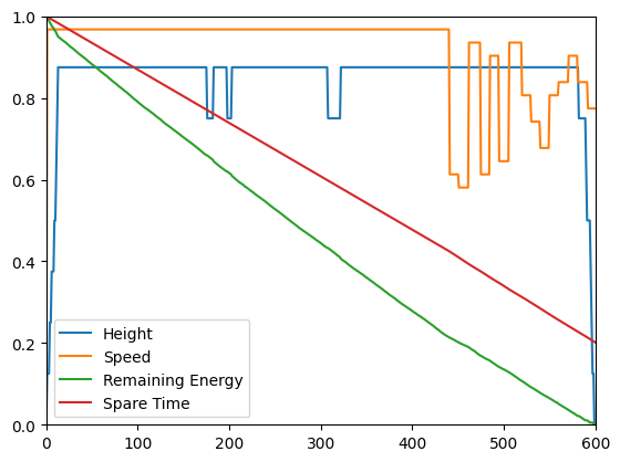
Best time preserving trajectory:

trajs.plot_traj(-1)

Balanced trajectory:

nt, _ = trajs.trajs.shape
trajs.plot_traj(nt // 2)